Pattern formation on a finite disk using the SH35 equation
Author: Nicolás Verschueren
Contents
- Summary
- Installation notes for PDE2PATH
- Cubic-quintic Swift-Hohenberg model (SH35) on a finite disk
- SH35 in PDE2PATH
- Initialization and continuation of the trivial branch
- Switching branches from the trivial state
- Radial branch
- Wall branch
- Presentation of results
- Solutions on the full disk
- Concluding Remarks
- Troubleshooting
Summary
This document offers a hands-on approach to the continuation code PDE2PATH. We consider the Swift-Hohenberg model with a cubic-quintic nonlinearity (SH35) solved on a finite disk of radius  with no-flux (Neumann) boundary conditions. We investigate the possible bifurcations of the trivial branch
  . This document is the first part of the supplementary material of the paper Localized and extended patterns in the cubic-quintic Swift-Hohenberg equation on a disk by N.Verschueren, E. Knobloch and H. Uecker. The second part, consisting on a list of videos, can be accessed in this link. The html file that you are reading has been produced from the script index.m, using the command publish. The reader can run index.m (included in the repository) to obtain the output shown below.
Installation notes for PDE2PATH
For installation instructions, tutorials and the latest version of PDE2PATH; visit the official website here. In this document we assume that the user is on a machine with MATLAB (notice that it is also possible to run PDE2PATH without MATLAB, see the website for details).
As PDE2PATH keeps evolving, future versions might present compatibility issues with this script (index.m). To avoid this, all the files needed to run it (including a version of PDE2PATH) are hosted in the bitbucket repository here.
In order to install the materials, visit the repository website and download the whole repository as a zip, by clicking on the download option on the left bar (this might change in the future). When the repository is unzipped into a local folder, the directory tree has the structure
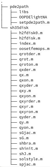
The two folders contain:
- pde2path/: a minimal version of PDE2PATH
- sh35disk/: the files used in what follows in this document.
Most names are self-explanatory. The script setpde2path.m must be executed succesfully to use PDE2PATH.
Please make sure you have PDE2PATH working on your machine before going any further with the demonstration.
Cubic-quintic Swift-Hohenberg model (SH35) on a finite disk
In what follows, we study the SH35 model

The variable  is defined over a disk of radius given by
![$$\Omega_1=\{\mathbf{x}\in (\rho,\phi)|\rho\in[0,R],\phi\in[0,2\pi]\},$$](index_eq05549450505803787802.png)
although a sector of a disk (a slice) will also be considered (more details below). The boundary conditions of this problem are given by

Since the system is variational, we can focus on its time-independent solutions. More precisely, the system minimises the functional
![$$\mathcal{F}[u]=\int_\Omega\left(\frac{1}{2}[(q^2+\Delta)u]^2-\frac{\epsilon}{2}u^2-\frac{\nu}{4}u^4+\frac{1}{6}u^6 \right) d\mathbf{x}.$$](index_eq11003998338834921733.png)
Finally, notice that the trivial solution exists for all parameter values and
![$$ \mathcal{F}[0]=0.$$](index_eq05150047716617588761.png)
Although the system has 4 parameters ( ), we keep
  ,
,  ,
,  , and investigate the bifurcations when
  is varied.
SH35 in PDE2PATH
PDE2PATH requires that the problem under study is written in the following (F)inite (E)element (M)ethod formulation (see documentation for details and explanations)

where  is the active continuation parameter,
  is a vector containing a discrete approximation of the solution of the system at different points in the space. The matrices
  are to be defined. In this matrix F.E.M. formulation, the boundary conditions correspond to Neumann type (i.e. they match the problem under study). In the case of the SH35 equation, all derivatives are of even order and therefore the problem can be formulated as follows (see the SH23 tutorial in the tutorial section here for details).

Substituting these expressions into the FEM formulation leads to the equation

where we have used that 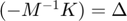 .
.
The two main steps in any PDE2PATH project are: initialization and iteration. At minimum, the following scripts are included in each project.
- sG.m The right hand side of the FEM formulation

- sGjac.m the Jacobian of
- oosetfemops.m the file with the FEM formulation. The definition of
- shinit.m the initialization file. This scripts calls all the above listed files and creates a structure of the problem
 .
.
Initialization and continuation of the trivial branch
The html that we are presenting (this document that you are looking at now), corresponds to the output of the script index.m. Hence, index.m can also be executed directly into MATLAB allowing exploration in the individual parts of the script.
Moving to the subdirectory local/pde2path, we set up PDE2PATH by calling the script setpde2path.m, then change directory (cd) into sh35disk/
clear;close all
format compact
cd ../pde2path/
setpde2path
cd ../sh35disk
pde2path, v2.9. Setting library path beginning with ~/tutorialdisk/pde2path
*** No additional libs put into path ***
When a PDE2PATH project is designed, the first task is to write the above listed files (e.g. sG.m, sGjac.m, etc) correctly (These files are already written and provided in the repository). Once this has been done, the code is ready to be used (initialized and iterated). Usually this is done on a separate script (often called commands cmds.m file). A possible initialization script is shown in the following cell. Each line contains a brief comment.
p=[]; %create the structure of the project
dswitch=2;% this corresponds to half the disc
lam=-0.01;% initial value of epsilon
nu=1.4; %initial value of nu
q=1; % initial value of q. This will not change
par=[lam nu q 0 0 0]; %vector with parameters
rad=14; %disk radius
nref=5; % fineness of discretization
p=shinit(p,dswitch,par,rad,nref);%initialize the structure p
plotsol(p,1,1,1); %meshplot (to inspect mesh)
p=setfn(p,'0h');%set the working directory
p.nc.ds=0.01;% initial stepsize for the continuation
p.nc.dsmax=0.1; %maximum stepsize for the continuation
p=cont(p,7); %continue the system for 7 steps
ans =
        8192           3
Problem directory name: 0h
creating directory 0h
step   epsilon     y-axis  residual  iter meth   ds       #-EV b(0)
   0   -0.01000  0.000e+00 0.00e+00    0     0.000e+00   0  0.000e+00
   1   -0.00900  0.000e+00 0.00e+00    0       0.00100   0  0.000e+00
   - 1 possible bif between -0.009 and 0.0010003, om=0
 mu_r=8.55829e-06, mu_i=0
<phi,psi>=0,BP
   2  -5.59326e-06 (BP, saved to 0h/bpt1.mat) bisection steps 10, last ds 4.88281e-06
   3    0.00100  0.000e+00 0.00e+00    0  nat    0.01000   3  0.000e+00
   - 1 possible bif between 0.0010003 and 0.0110006, om=0
mu_r=0.0028738, mu_i=0   - no convergence
   4    0.01100  0.000e+00 0.00e+00    0  nat    0.01000   2  0.000e+00
   - 1 possible bif between 0.0110006 and 0.0310012, om=0
 mu_r=7.36877e-06, mu_i=0
<phi,psi>=0,BP
   5  2.14892e-02 (BP, saved to 0h/bpt2.mat) bisection steps 10, last ds 9.76563e-06
   - also saved to 0h/pt5.mat
   6    0.03100  0.000e+00 0.00e+00    0  nat    0.02000   1  0.000e+00
   - 1 possible bif between 0.0310012 and 0.0510018, om=0
 mu_r=-1.6043e-05, mu_i=0
<phi,psi>=0,BP
   7  3.21926e-02 (BP, saved to 0h/bpt3.mat) bisection steps 10, last ds -9.76563e-06
   8    0.05100  0.000e+00 0.00e+00    0  nat    0.02000   4  0.000e+00
Timing: total=13.2271, av.step=1.47449, av.newton=0.00563387, av.spcalc=0.0848556

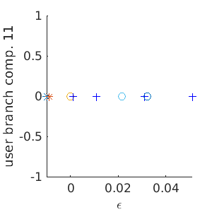
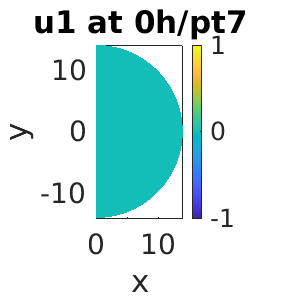
The previous snippet of code produces 7 rows with the relevant information of the continuation. This output will be supressed in the future continuations performed on this document. The bifurcation diagram on the left summarises the continuation information. The 7 continuation points are distinguished as stable (*) unstable (+) and bifurcation (o) points using different symbols (folds are also marked with an (x) see below). On the right, we can see a representation of the component  of the solution. Notice that one bifurcation point was found in this way. We can use this point to switch into nontrivial branches.
Switching branches from the trivial state
In this problem, the trivial branch is connected to several solutions for  , The next cell illustrates some possibilities.
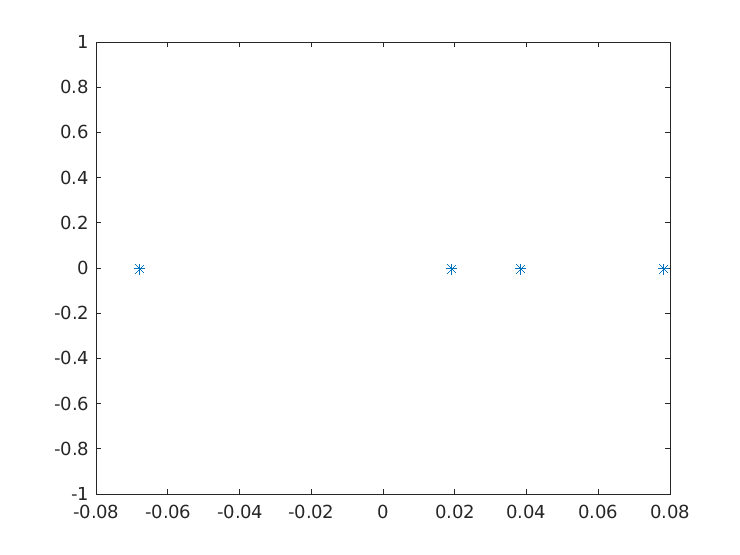
aux.m=6; %number of eigenvalues to look at\
aux.besw=0; % don't derive/solve bifurcation equations
possibles=cswibra('0h','bpt1',aux);
possibles.nc.eigref=-1; % compute eigenvalues closest to eigref; set negative to not miss unstable eigenvalues
using m=6
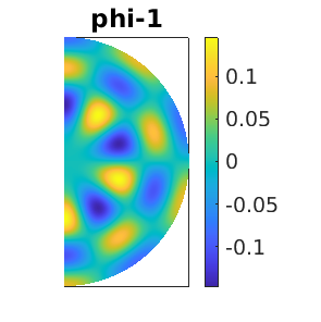
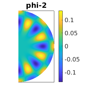
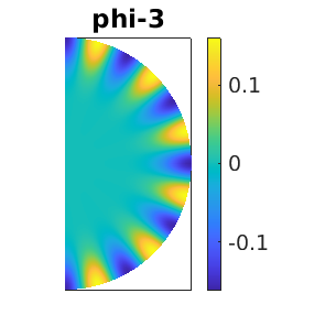
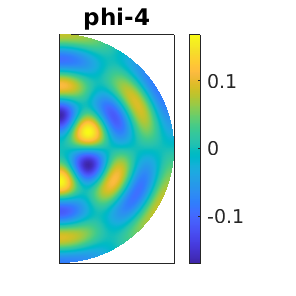
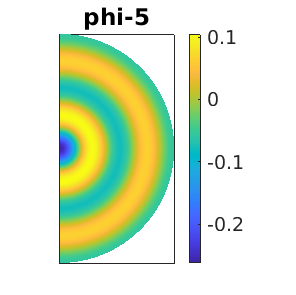
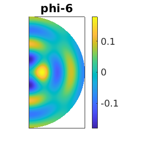
The possible directions of continuation are listed as  . We investigate two of them: the daisy (
 ) and radial (
 ) branches. The process to investigate other possibilites is analogous and we encourage the reader to experiment.
Radial branch
Once the different directions have been identified, continuation of the radial branch is done by
p=gentau(possibles,[0 0 0 0 1],'radial'); %we are taking the 5th vector of the possibles and choosing 'radial' as the new directory
close all;
screenlayout(p); %close figures
p.sw.bifcheck=0; %we are not interested in detecting bifurcations, so we disable this feature to increase the speed.
p=cont(p,5); %notice that up to this point, the solution is localized in the center and consequently it is free to move...
p=qyon(p); %We introduce a phase condition to eliminate the symmetry, allowing continuation (see the documentation for details)
p.sol.restart=1; %recalculating the tangential vector
p.sol.ds=-0.01;%continuation step, we invert the direction
p.nc.neig=30; %number of eigenvalues computed
p.sw.verb=2; %maximum verbosity
p=cont(p,30); %continuation on the radial branch for 30 extra steps
Problem directory name: radial
creating directory radial
step   epsilon     y-axis  residual  iter meth   ds       #-EV b(0)
   1    0.00843    0.00961 1.05e-10    2  arc    0.01000   4    0.16863
  35    0.32909    0.98728 1.01e-11    2  nat   -0.08000   0   17.32325
Timing: total=32.8149, av.step=0.91856, av.newton=0.238479, av.spcalc=0.399637
Wall branch
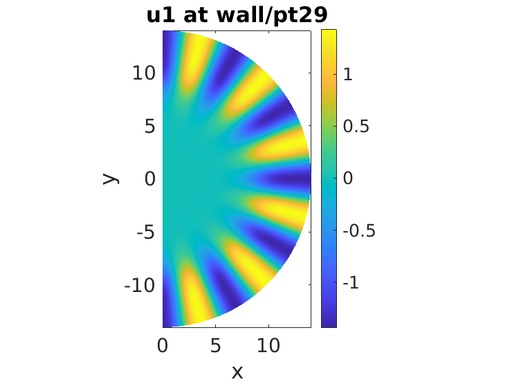
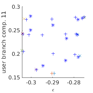
Similarly, we can do continuation of the wall branch. Since we are interested also in secondary bifurcations, we turn the detection of bifurcation points (p.sw.bifcheck=1) for the first ten continuation points and subsequently complete the wall branch without detecting bifurcation points (to increase the speed as shown in the radial branch case).
close all;%close the figures
p=gentau(possibles,[0 0 1],'wall'); %we are taking the 5th vector of the possibles and choosing 'radial' as the new directory
p.sw.bifcheck=1; % at start of branch we are interested in bifurcations
p.sw.verb=2;  % some additional output (plotting eigenvalues to Fig.6)
p=cont(p,10); %
p.sw.bifcheck=0; % switch off bif.detection for the rest of the branch
p=cont(p,20);
Problem directory name: wall
creating directory wall
step   epsilon     y-axis  residual  iter meth   ds       #-EV b(0)
   stepsizecontrol: dlam=-0.000369451, res=1.94477e-09, increasing ds to 0.02
   1   -0.00038    0.01058 1.94e-09    1  arc    0.01000   1    0.18560
  30    0.42287    0.75194 4.68e-10    2  nat    0.08000   4   13.19382
Timing: total=18.5784, av.step=0.757559, av.newton=0.18985, av.spcalc=0.336649
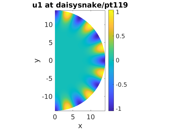
As shown in the manuscript, the secondary bifurcation leads to localization and snaking in the angular direction: daisy snaking. In this case we know a priori that there is a single unstable direction and therefore there is no need to use cswibra and gentau. Instead, we simply use swibra:
clf(2);
p=swibra('wall','bpt1','daisysnake');
p.sw.bifcheck=0;
p=cont(p,120);
lam=-0.010376; 4 smallest eigenvalues: 1.7892e-06   0.0040375   0.0053953   -0.021309
zero eigenvalue is 1.78919e-06
d/ds(lam)=-0.469648
Problem directory name: daisysnake
creating directory daisysnake
step   epsilon     y-axis  residual  iter meth   ds       #-EV b(0)
   stepsizecontrol: dlam=-0.00187885, res=2.67936e-09, increasing ds to 0.02
   1   -0.01225    0.04360 2.68e-09    2  arc    0.01000   1    0.76495
 120   -0.37526    0.33587 7.04e-14    4  arc    0.01000   1    5.89338
Timing: total=158.117, av.step=1.17061, av.newton=0.431254, av.spcalc=0.323186
Presentation of results
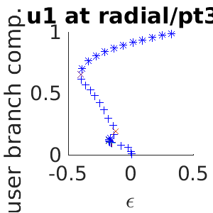
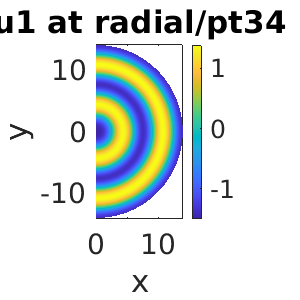
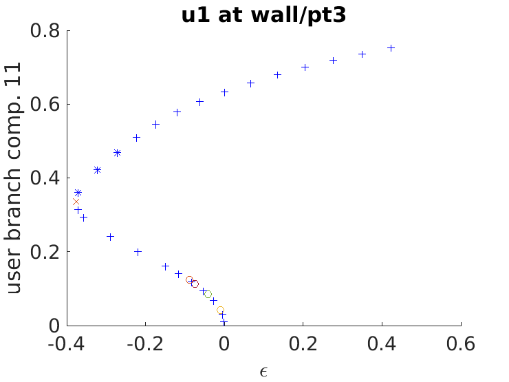
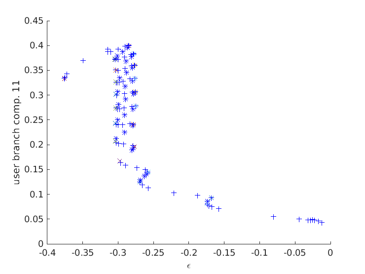
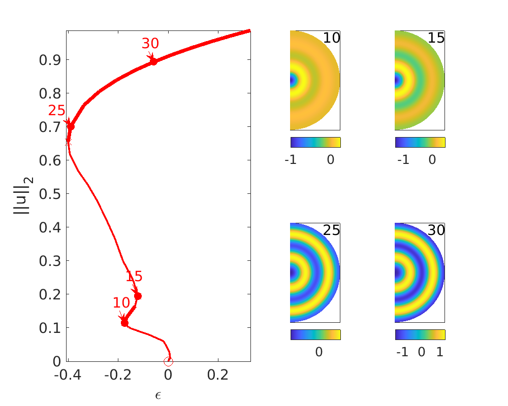
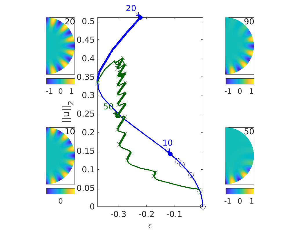
PDE2PATH includes the functions plotsol and plotbra to represent the solutions and solution branch, respectively. The following cell illustrates some of the capabilities of these functions (see the tutorial called plot in the documentation for details) by showing two figures: one for the radial branch and one with the daisy and daisy snaking behavior. In each case, the bifurcation diagram is presented with four sample solutions marked and illustrated on the sides
keep pphome
close all
f=10; %figure number radial
figure(f);
subplot(2,4,[1 2 5 6])
plotbra('radial','cl','r','lab',[10,15,25,30],'wnr',f)
ylabel('||u||_2')
subplot(2,4,3);plotsol('radial','pt10',f);solstyle('10')
subplot(2,4,4);plotsol('radial','pt15',f);solstyle('15')
subplot(2,4,7);plotsol('radial','pt25',f);solstyle('25')
subplot(2,4,8);plotsol('radial','pt30',f);solstyle('30')
set(gcf,'Position',[200 300 1000 800])
f=11;figure(f)%wall
subplot(2,4,[2 3 6 7])
plotbra('wall','cl','b','lab',[10, 20],'wnr',f,'lp',20)
plotbra('daisysnake','cl',p2pc('g1'),'lab',[50,90],'wnr',f)
ylabel('||u||_2')
subplot(2,4,5);plotsol('wall','pt10',f);solstyle('10')
subplot(2,4,1);plotsol('wall','pt20',f);solstyle('20')
subplot(2,4,8);plotsol('daisysnake','pt50',f);solstyle('50')
subplot(2,4,4);plotsol('daisysnake','pt90',f);solstyle('90')
set(gcf,'Position',[200 300 1000 800])
lam=-0.173531
lam=-0.121827
lam=-0.389833
lam=-0.0572852
lam=-0.11578
lam=-0.222289
lam=-0.30392
lam=-0.290178
Solutions on the full disk
So far we have used a sector of the full disk (half a disk). As explained on the paper, using a sector has many advantages (e.g. reduced the number of points, most solutions can be continued with no phase condition, there is a filter for the possible solutions allowed). A drawback is that stability is computed for the sector and some solutions will be stable on the sector and unstable on the full disk.
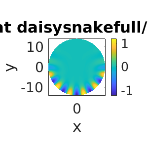
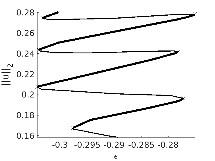
In order to perform continuation on the full disk, the script shinit.m includes the case of the full disk when ndim=5. Hence, one option is to re-run the above code with ndim=5 instead of 6. Alternatively, we can reflect a given solutions from half-disk into the full-disk. A simple script to perform such a task, called h2fdisk.m, has been provided. We illustrate the continuation of the localized daisies on the full disk.
keep pphome; close all;
p0=[]; %Firstly, we creat a structure with a domain for the full disk
dsw=1;%full disk
lam=-0.01;
nu=1.4;
q=1;
par=[lam nu q 0 0 0];
rad=14;
nref=5;
p0=shinit(p0,dsw,par,rad,nref);
p=h2fdisk('daisysnake','pt30',p0,'daisysnakefull'); %pt30 from half domain is mirrored
p=resetc(p);
p.sw.bifcheck=0;
p=qroton(p); % a phase condition is added to avoid rotation
p.sol.ds=-p.sol.ds;
p=cont(p,30);
plotbra('daisysnakefull');
ylabel('||u||_2')
ans =
       16384           3
Problem directory name: daisysnakefull
creating directory daisysnakefull
Problem directory name: daisysnakefull
step   epsilon     y-axis  residual  iter meth   ds       #-EV b(0)
   0   -0.28923    0.15857 0.00e+00    0     0.000e+00   2    3.93470
   1   -0.29023    0.15901 0.00e+00    0      -0.00100   2    3.94576
  31   -0.30029    0.28037 5.68e-14    4  arc   -0.01000   0    6.95711
Timing: total=85.4887, av.step=2.58877, av.newton=1.03659, av.spcalc=0.363829

Concluding Remarks
In this document, we have illustrated the first steps on using the code PDE2PATH, considering the SH35 Model on a finite disk as an example. The aim of the document is not to be thorough, but to provide a brief introduction to PDE2PATH as well as illustrate how to obtain some of the results presented in the paper. Hopefully this can be the starting point for many future users of PDE2PATH.
Several aspects of PDE2PATH, some of them included in the paper, were not investigated at all here. We briefly mention some possible future investigations.
The last continuation on the full disk, shows how PDE2PATH slows down as the number of points increases. It is possible to increase the speed by installing and linking the library ilupack. This step can vary between operative systems and we suggest the interested reader to refer to the official documentation. Once this library is working, the routine can be called via the function setilup and continuation can be perfomed as shown before.
Throughout this document, we explored numerical continuation in . It is of course possible to perform continuation in any other parameter as well as changing the parameter (see swipar in the documentation) at any continuation point. Moreover continuation of special points is possible (e.g. continuation of folds, Hopf bifurcation points, bifurcation points). For such cases, additional derivatives should be provided. It is also possible to: implement different boundary conditions, perform direct numerical simulation of solutions, redistribute (remesh) the points in the domain, to name just a few. All the above mentioned features are explained well in the repesctive tutorials.
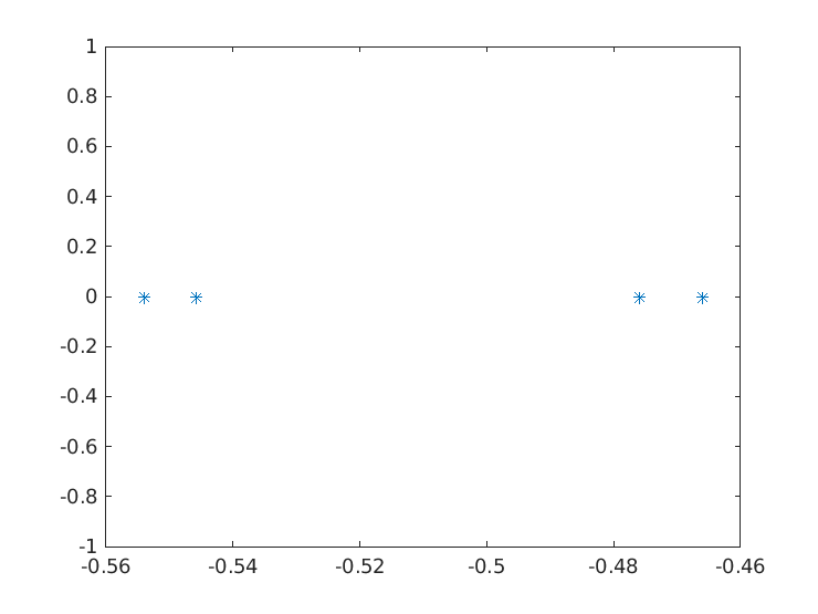
Troubleshooting
If you encounter any discrepancies between what is reported here and the output of your computer, this can be due to the eigenvectors sorted in a different way. For primary bifurcations, make sure that the eigenvectors look like those reported here. The same phenomenon can happen with the bifurcations from the wall branch. If problems persist, feel free to send me an email to nv13699@my.bristol.ac.uk. Also feedback (e.g. suggestions to improve this document, typos, etc) is more than welcome.